🅱️The current price of Bitcoin is about $60,508 (daily closing price):
According to the OLS regression model, the price is 21.7% below fair value, or $77,464 (mean).
Based on the modal regression model, the excess over fair value is 38.3%, or $43,852 (modal).
Using the 50th percentile regression model, this represents a 10.5% discount to fair value, or $67,754 (median).
The median as a reference point provides the best balance of robustness relative to Bitcoin’s inherent power law, and is the most appropriate given Bitcoin’s skewness and heteroskedasticity.
♣️ Let’s review three basic statistical metrics — mean, median, and mode — and apply them to an assessment of Bitcoin’s “fair value” price based on its well-established power-law behavior.
>>Mean: This trend is determined by performing an Ordinary Least Squares (OLS) regression, where the squared error of all price data is minimized.
>> Weakness of the mean: The OLS mean is an “average” that places a lot of weight on large errors and is therefore more susceptible to large biases and outliers. This also applies here, as Bitcoin’s biases/residuals are heavily skewed (right graph). It is also best when the distribution of errors/biases is assumed to not change over time (or be “homoskedastic”; Bitcoin’s residuals are “heteroskedastic”, meaning they decrease over time).
>>Median: To capture the median trend, quantile regression is used at the 50th percentile - meaning 50% of the price data is below this line and 50% is above this line. In this case, the error reduction is absolute, not squared.
>> Strength of the Median: The median is the middle point of all the data at any given time. It is relatively resistant to large deviations (which occur less frequently), so it tracks the "central tendency" of the price distribution better than the mean. In short, it is less affected by the skewness or heteroskedasticity of the distribution.
>>Mode: The mode is simply the value that occurs most often in a distribution of values; so if there is a distinct peak, the mode will be that peak.
>> Strengths of Patterns: Patterns will always reflect the values that occur most often (in this case, we are talking about the residuals of Bitcoin’s power law — “the line you can’t ignore”), and it is clear from analyzing the data that there is a support line that the price rarely breaks below, and even when it does, it is short-lived. The pattern is very good at tracking this line. It is also extremely resilient to large deviations (think FOMO bubbles) and outliers.
♣️Mode’s weakness: We know, in fact, that these FOMO bubbles do happen; it’s part of seasonality, the interface between standard pricing of assets and human psychosocial, political and economic cycles. Modes don’t care about any of that; therefore, modes will generally undervalue assets with respect to this known seasonality.
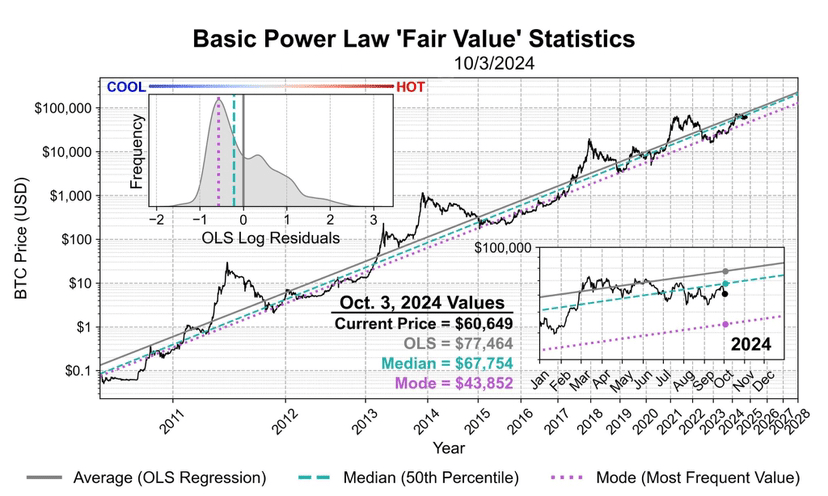
♣️Application in chart:
The main chart shows the entire price history of Bitcoin on a log-log scale (the line you can’t ignore). The inset on the lower right zooms in on the year 2024 and shows an overlay of the OLS regression (solid grey), the 50% percentile regression (dashed turquoise), and the modal regression (dashed purple).
In the top left inset, you can see the frequency distribution of Bitcoin’s log residuals. As a guide, the red/blue arrows illustrate how “hot” or “cold” BTC’s price is depending on the size of the residual — which can be thought of as the “shadow” of all the price data along the straight power law line.
You can also visualize each model - note the difference in "central tendency" between OLS, median, and mode.
Thanks for sticking around to read this long explanation - would you like to see this updated regularly? Let me know!