🐮 Understand Bubblemaps in 60 seconds (super simple)
#Bubblemaps What is it?
Draw the 'top 250 holding addresses' as bubbles: bigger bubble = more coins; lines between bubbles = mutual transfers. You can clearly see the concentration (whether a few are holding the majority of the coins) and the correlation (whether seemingly dispersed wallets are actually interconnected).
Two key functions
Magic Nodes: Add originally non-top 250 addresses that are responsible for 'linking funds' into the diagram (e.g., common upstream USDT/USDC sources, common inflows).
Time Travel: 'Rewind' the map to the release date, before the listing, or before a significant price surge, to compare whether the concentration was evident early or if there was a gathering before news.
Bubblemaps turn 'supply auditing' into a diagram that everyone can understand. During the meme coin craze, it helps you see distribution first, then discuss technical aspects, significantly reducing the chances of buying into inner control or potential exit scams.
🐮 3 minutes to practical action: How to read a BubbleMap
Step 1|Open the chart and filter
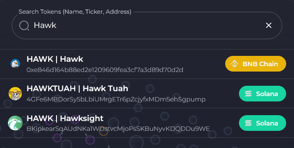
Search for token contract (input Hawk) → Open the map.
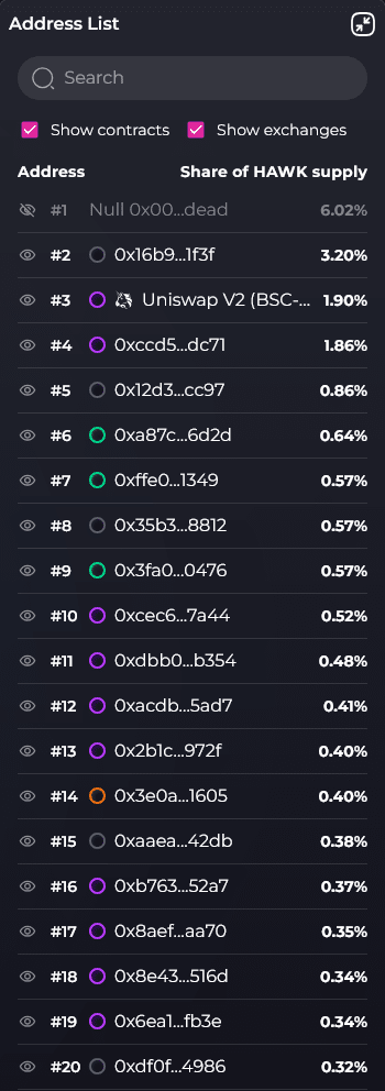
Check Show contracts / Show exchanges in the right column, marking LP, contract, and exchange addresses that cannot be freely shipped to avoid misjudging as 'whales'.
Step 2|Health Scan
Look at the right column Top list: is there a single address >10%? Do the Top 5 **>25%**? (The higher, the more concentrated)
Does the map show a 'single super large cluster' occupying double digits?
Is there a large amount in the outer circle?small bubbles(long tail retail)?
It all looks very dispersed!
Step 3|Magic Nodes (60 seconds)
After opening, check if there are common upstreams linking multiple large bubbles.
If it originally looked dispersed, but suddenly 'gathers into one', that is a strong signal of hidden associations.
Step 4|Time Travel
Rewind to the release day, before listing/significant announcements, or 24–48H before the last major surge:
Was there concentration early on?
Was there a sudden gathering before news?
Was there a quick outflow after inflow?
🐮 Practical: Step by step interpretation using #Bubblemaps Hawk chart
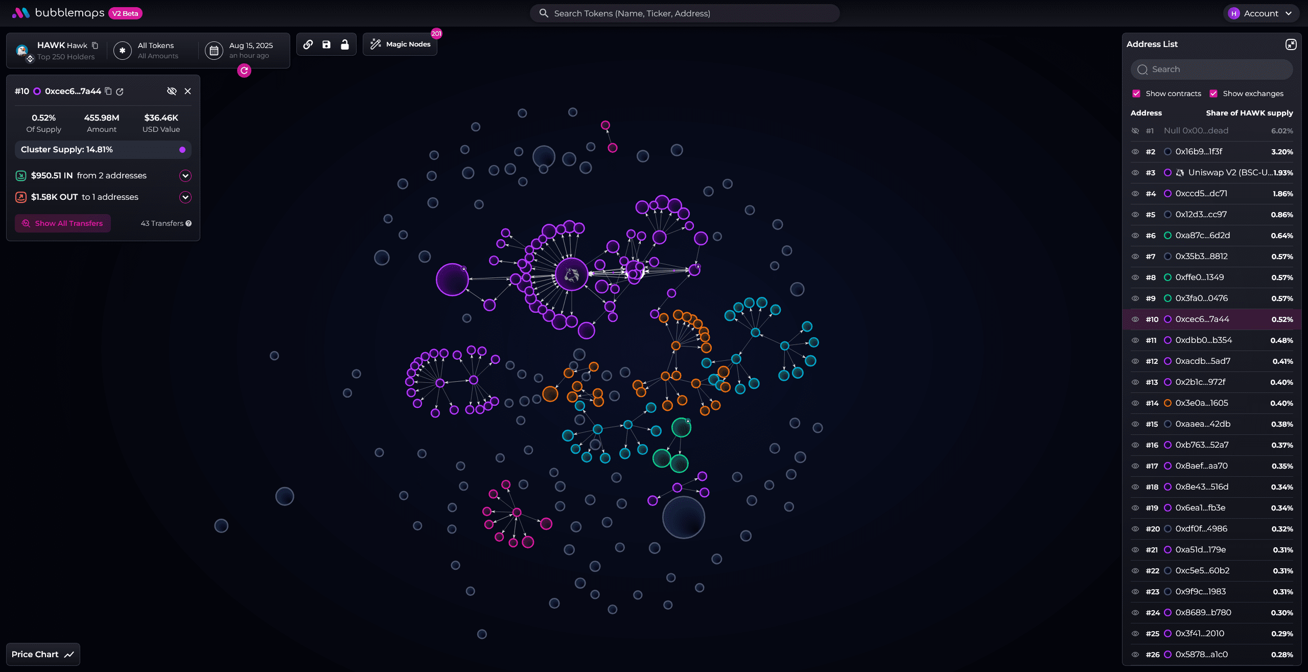
1) Initial observations before opening Magic Nodes (A)
Right column Top:
#1 Null 0x00…dead ≈ 6.02% (Black Hole/Demolished, not accessible)
#3 Uniswap V2 … ≈ 1.93% (LP/Contract type)
Most others are in the 0.2%–0.6% range. At a glance, there is no overwhelming super whale.
Chart structure:
There aremultiple medium clusters(colored differently), outer circlelong tail small bubblesquite a few.
First impression conclusion: If you only look at this chart, Hawk resembles 'multiple clusters coexisting, with no single point having 10% extreme concentration', risk-neutral and relatively stable.
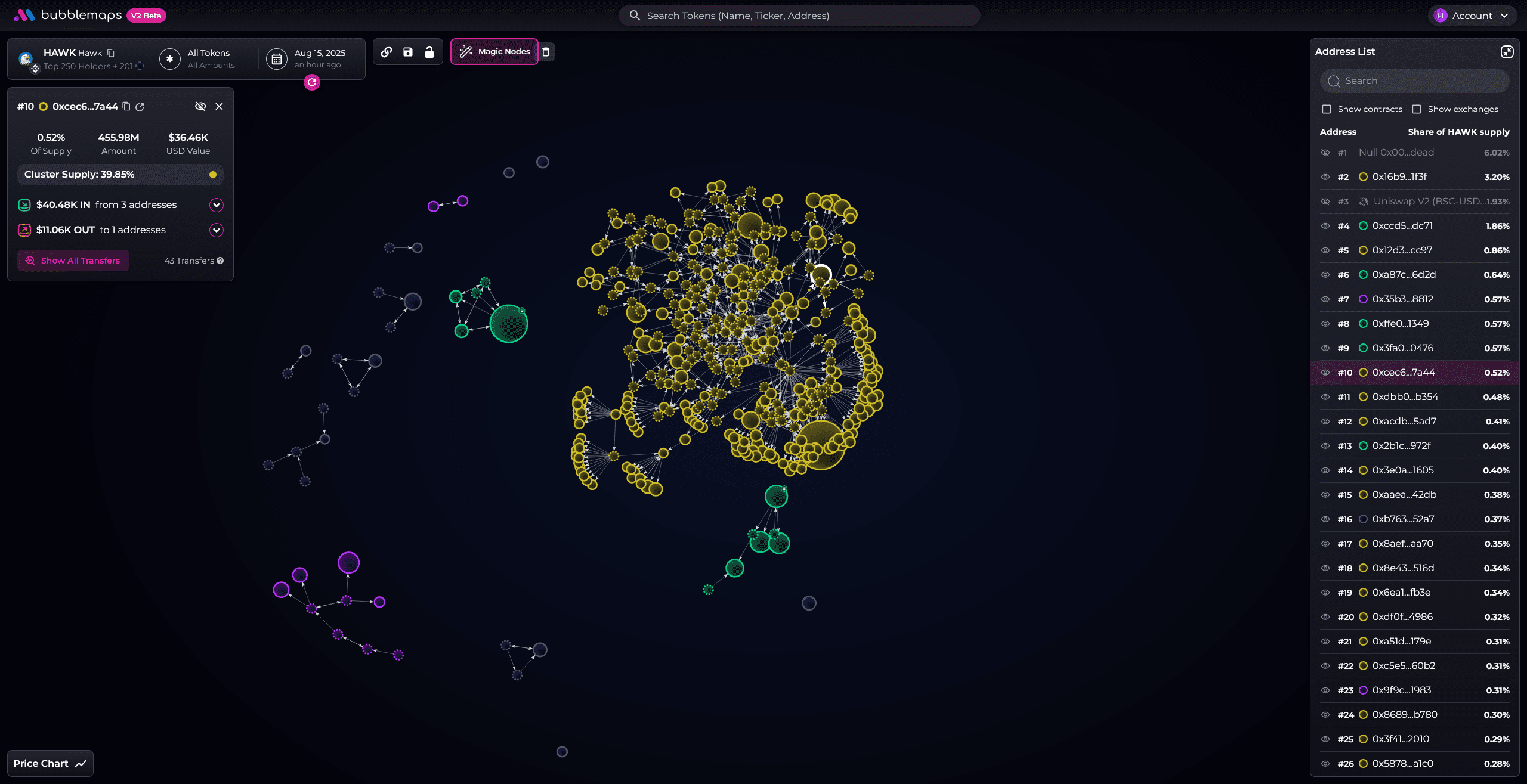
2) Key changes after opening Magic Nodes (B)
The same #10 info card appears:
Cluster Supply: ≈ 39.85% (← This is the key to this analysis)
Single points are still at 0.52%, but the entire group of that color (the related clusters connected by Magic Nodes) totals nearly 40% of the supply.
Also shows $40.48K IN (3 addresses), $11.06K OUT (1 address), totaling 43 transactions.
Visual representation:
A whole arealarge yellow clusteroccupying the center of the screen, with very dense internal connections, not just a few points connected by chance, but multiple points beingcommon hubsinterconnectedassociation network.
Key Interpretation
Magic Nodes reveal hidden associations: many 'common upstream/inflow' addresses not originally in the Top 250 or with zero balance were added, thus weaving seemingly dispersed multiple wallets into one.
39.85% large clusters = high concentration risk: even if the right column Top list appears dispersed, once you include hidden nodes, the chips that can be influenced may be cooperated by the same group of people.
This does not equate to the legal definition of 'the same person', but in terms of trading risk, the behavioral correlation is significant enough to constitute a major signal.
3) Use 'traffic lights' to grade Hawk
Red light (increased risk weight)
Single large cluster after Magic Nodes ≈ 39.85%.
High internal connection density, suspected common upstream/inflow.
Green light (relatively positive)
There are dead addresses ~6% and LP/contracts in the front row (functional/non-accessible).
The single point proportion in the right column Top list is not extreme.
Preliminary conclusion: Concentration = high. Further analysis can use Time Travel and Transfers' historical/counterparty details, but based solely on the current chart, trading should adopt 'conservative positioning + strict risk control'.


